Using the Global Embeddings in Your Own Analysis
OlmoEarth publishes annual embeddings for the Earth's land surface at 10 m resolution, free to download from Source Cooperative. This page explains what the dataset contains and how to export an area of interest as a GeoTIFF you can open in QGIS or any other GIS application.
If you only want to browse the embeddings or run a similarity search, the Embeddings Explorer does that in your browser with no code for an area up to about 2000 km².
What an embedding is
An embedding is a set of numbers that summarizes what satellites observed at one pixel over a full year. It combines Sentinel-1 radar, Sentinel-2 optical, and Landsat 8/9 imagery.
In GIS terms, the dataset behaves like a raster with 128 bands. Unlike Sentinel-2's red or near-infrared bands, no single band has a physical meaning. What matters is that pixels with similar surfaces,
such as two cornfields or two wetlands, have similar values across the bands. That makes embeddings useful as inputs for classification, similarity search, and change detection.
The first 64 bands also work as a complete embedding on their own. They perform well for most tasks and are half the size to download.
What's in the dataset
| Resolution | 10 m |
| Years | 2017 to 2025, one embedding per calendar year |
| Bands | 128 (or the first 64 on their own) |
| Coverage | Land and coastal water from 59.5°S to 83.6°N, excluding Antarctica |
| Format | Zarr, one array per UTM zone |
| Access | Public and anonymous: no account or API key |
| License | OlmoEarth Artifact License |
What Zarr is
Zarr is a format for storing very large multi-band rasters in the cloud. Instead of one large file, the raster is split into many small tiles that are stored separately. Software reads only the tiles that cover your area, so you never download the whole dataset. If you have used Cloud-Optimized GeoTIFFs (COG files), the idea is the same.
You don't need to understand Zarr in depth to use this dataset. The script below reads the tiles for your area and writes a standard GeoTIFF.
How the data is organized
- One array per UTM zone. The world is split into the 60 UTM zones,
utm01throughutm60, and each zone is stored in its own projection. Your area's zone number isint((longitude + 180) / 6) + 1. Minnesota, for example, is mostly in zone 15. - Each zone has four dimensions: year, band, northing, and easting.
- Values are compressed whole numbers. To keep the dataset small, each value is stored as a whole number from -127 to 127 on a curved scale. Convert the values back to decimals before doing any math with them. The script below does this for you.
- -128 means no data: either the pixel is outside the coverage area, or there was no usable Sentinel-2 imagery for it that year. It does not necessarily mean there is no land.
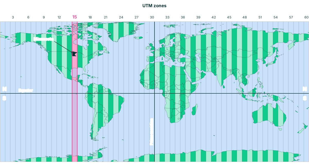 For illustration only, zone and border positions are approximate
Export an area as a GeoTIFF
1. Install Python packages
You need Python 3. Create a virtual environment (a private folder for this project's packages), then install the packages into it:
    python3 -m venv olmoearth-env
    source olmoearth-env/bin/activate
    pip install "zarr>=3" obstore pyproj numpy rasterio
On Windows, activate the environment with olmoearth-env\Scripts\activate instead. Run the activate command again each time you want to export embeddings in a new terminal.
2. Set your area of interest
WEST, SOUTH, EAST, NORTH are the four edges of a rectangle around your area. Two of them are longitudes (the left and right edges) and two are latitudes (the bottom and top edges) in decimal degrees. Together they’re the same as two lat/lon corners: the bottom-left corner is (SOUTH, WEST) and the top-right corner is (NORTH, EAST).
Any GIS application can give you these numbers: they’re the extent, or bounding box, of a layer covering your area. Make sure the layer is in WGS84 (EPSG:4326) so the extent is in decimal degrees. For example, in QGIS, open Layer Properties → Information and find Extent. It’s listed as xmin,ymin : xmax,ymax, which is WEST,SOUTH : EAST,NORTH.
If you don’t have a layer for your area, you can draw a box on a web map such as bboxfinder and copy the coordinates it lists in west,south,east,north order. Make sure to use the right coordinate system!
The script's example covers about 8 km by 9 km of Minneapolis, Minnesota:
WEST, SOUTH, EAST, NORTH = -93.30, 44.90, -93.20, 44.98
Choosing a size
Start small. Each year you export is about 2.5 MB per square kilometer at 64 bands, or about 5 MB at 128 bands, before compression. The Minneapolis example is about 180 MB. An area the size of Minnesota, about 225,000 km², would be over 500 GB for a single year.
For large regions, export several smaller areas, or sample embeddings only at your labeled points instead of exporting a full raster.
Staying within one UTM zone
The embeddings are stored by UTM zone, each 6 degrees of longitude wide. The script exports from one zone at a time, chosen by your area's western edge. If your area crosses into the next zone, the script prints a warning and exports only the part inside the first zone. Run it again for each additional zone, with a bounding box covering the part of your area inside that zone.
Minnesota, for example, falls mostly in zone 15, but a narrow strip along its western edge is in zone 14, and the tip of the Arrowhead in the northeast is in zone 16.
3. Run the export script
Set your area of interest and the year, then run the script. Note that this script is for a single year. To export another year, change YEAR and run it again. The output file name includes the year, so each run writes a new file instead of overwriting the last one. It writes a 64-band GeoTIFF in your area's UTM projection.
import numpy as np
import rasterio
import zarr
from obstore.store import S3Store
from pyproj import Transformer
from rasterio.transform import Affine

# --- Settings: change these for your area, year, and band count (64 or 128) ---

WEST, SOUTH, EAST, NORTH = -93.30, 44.90, -93.20, 44.98
YEAR = 2025
BANDS = 64
OUTPUT = f"olmoearth_embeddings_{YEAR}.tif"

# --- Connect to the dataset on Source Cooperative ---

# Download only the tiles you need, without merging nearby requests.
zarr.config.set({"array.sharding_coalesce_max_gap_bytes": 0})

# The dataset is public, so no account or credentials are needed.
s3 = S3Store.from_url(
    "s3://olmoearth/olmoearth-v1-3-embeddings/embeddings.zarr",
    endpoint="https://data.source.coop",
    skip_signature=True,
)
root = zarr.open_group(zarr.storage.ObjectStore(s3, read_only=True), mode="r")

# --- Find the UTM zone for your area ---

# Each UTM zone is 6 degrees of longitude wide, numbered from 1 at 180°W.
zone_number = int((WEST + 180) // 6) + 1
if int((EAST + 180) // 6) + 1 != zone_number:
    print(f"Warning: your area crosses a UTM zone boundary. Only the part in zone {zone_number} will be exported.")

zone = root[f"utm{zone_number:02d}"]
crs = zone.attrs["proj:code"]

# --- Convert your bounding box from latitude/longitude to UTM meters ---

# Transform all four corners, since a box in lat/lon isn't a perfect rectangle in UTM.
to_utm = Transformer.from_crs("EPSG:4326", crs, always_xy=True)
xs, ys = to_utm.transform([WEST, EAST, WEST, EAST], [SOUTH, SOUTH, NORTH, NORTH])

# --- Convert UTM meters to row and column numbers in the zone's grid ---

# The grid's top-left corner (c, f) and pixel size in meters (a, e) come from the dataset.
a, _, c, _, e, f = zone.attrs["spatial:transform"]
col0, col1 = int((min(xs) - c) / a), int((max(xs) - c) / a) + 1
row0, row1 = int((max(ys) - f) / e), int((min(ys) - f) / e) + 1

# --- Download the embeddings for your area and year ---

t = list(zone["time"][:]).index(YEAR)
q = zone["embeddings"][t, 0:BANDS, row0:row1, col0:col1]

# Stop if there are no embeddings for this area and year yet (every pixel is -128, the no-data value).
if (q == -128).all():
    raise SystemExit(f"No embeddings for this area in {YEAR} yet.")

# --- Convert the stored whole numbers back to decimal values ---

# -128 marks no data and becomes blank (NaN), so it can't affect later calculations.
values = np.where(q == -128, np.nan, q).astype("float32")
values = (np.abs(values) / 127.5) ** 2.0 * np.sign(values)

# --- Save as a GeoTIFF with one band per embedding dimension ---

# Where your area's top-left corner sits on the map, so the GeoTIFF lines up in QGIS.
transform = Affine(a, 0, c + col0 * a, 0, e, f + row0 * e)

with rasterio.open(
    OUTPUT, "w", driver="GTiff",
    height=values.shape[1], width=values.shape[2], count=values.shape[0],
    dtype="float32", crs=crs, nodata=np.nan, compress="deflate",
    transform=transform,
) as dst:
    dst.write(values)

print(f"Saved {OUTPUT}")
Plan for file size. At 64 bands, the output is about 2.5 MB per square kilometer before compression, or about 5 MB at 128 bands. A 2,000 km² county at 64 bands is roughly 5 GB, so start with a small area.
4. Open it in a GIS application
Open the GeoTIFF in your GIS application as a raster layer. Most GIS applications display the first three bands as red, green, and blue. The colors have no physical meaning, but areas with similar surfaces will look similar, which is a quick way to confirm the export worked.
What to do next
- Attach embeddings to your labeled points. Use QGIS's Sample raster values tool to add the 64 band values to each point. The result is a table you can use to train a classifier.
- Classify, search, or detect change. The embeddings tutorial has working code for classification, similarity search, change detection, and clustering.
- Train a custom model in Studio instead. If you have labels but don't want to write code, fine-tune a model in OlmoEarth Studio.
Things that can trip you up
- Convert the values before doing math. The stored values are on a curved scale, so averages or distances on the raw numbers are wrong. The script handles this.
- Areas that cross a UTM zone boundary need one export per zone. The script warns you when this happens. Reproject the exports to a common grid before merging them.
- Southern-hemisphere areas have negative northings. Every zone uses the northern UTM projection, so locations south of the equator have negative y values. PROJ handles this correctly, but some tools may not.
- Don't mix 64-band and 128-band embeddings in the same analysis. Use the same BANDS setting for every export.
- Blank pixels don’t always mean water or missing land. A pixel is blank when no embedding was computed for it, either because it’s outside the dataset’s coverage or because there wasn’t enough usable Sentinel-2 imagery that year.
- For cosine similarity, normalize the vectors first. They aren't scaled to a length of 1.
- A narrow strip along the 180° meridian has no embeddings in zones 1 and 60.
Citation
If you use this dataset, please cite the OlmoEarth v1.3 Embeddings technical report. The BibTeX entry is in the dataset README.