How OlmoEarth Studio Works
This page walks through the OlmoEarth Studio workflow, from labeled data to predictions you can use. The examples come from a burn scar mapping project that classifies burned and unburned land from Sentinel-2 imagery, trained on more than 4,000 fire perimeter polygons. This dataset went through a few iterations to make it model-ready. To learn more about how to go from raw dataset to model-ready, please see our article on Getting a Dataset Ready for Modeling.
1. Upload and annotate your data
Start by uploading labeled points or polygons as a CSV or GeoJSON file, or by annotating directly on satellite imagery in Studio. Each label records what is at a location and when it was observed.
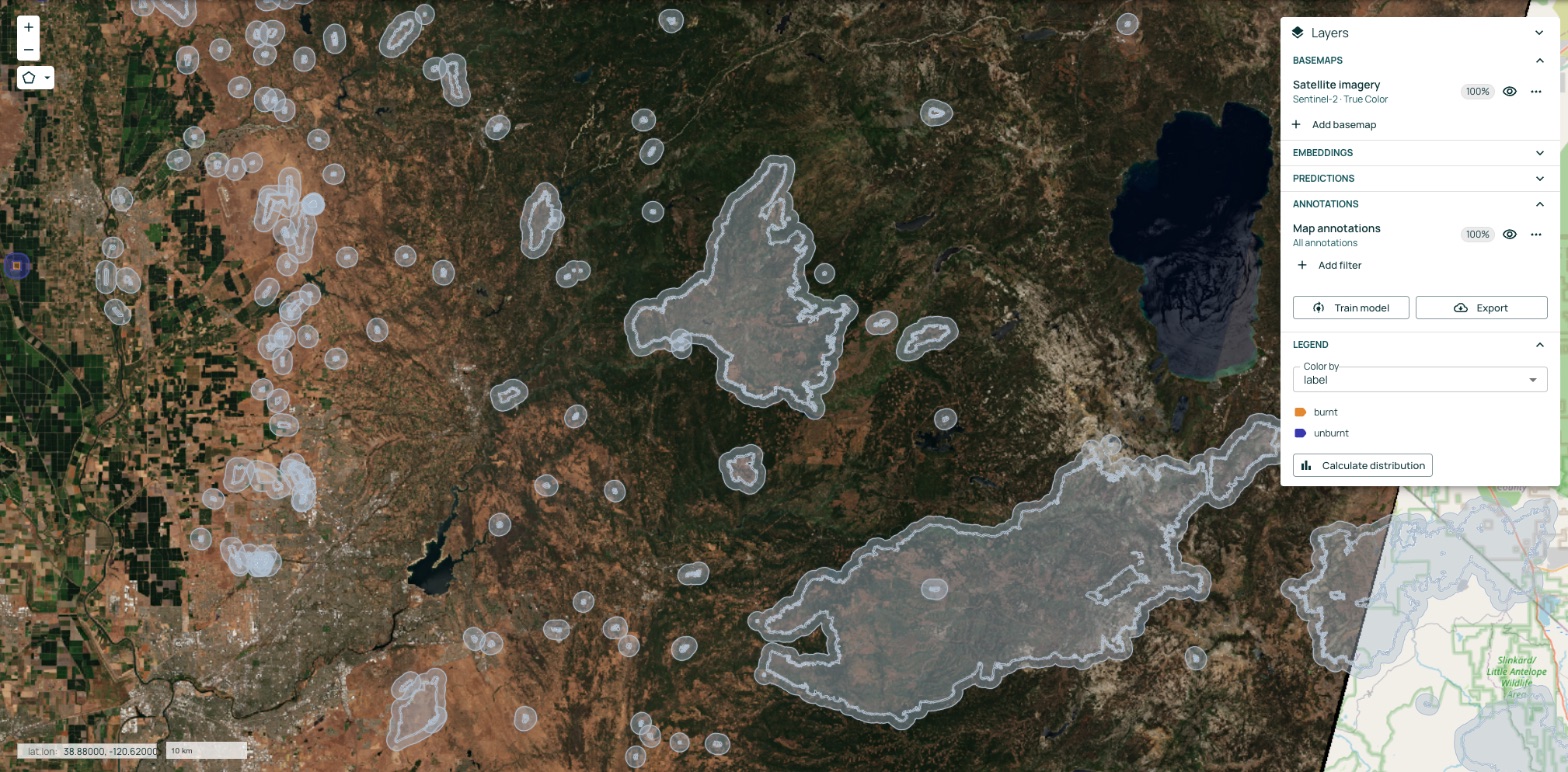
For file formats and required fields, see Training Data Requirements.
2. Fine-tune a new model
Studio fine-tunes a new model on top of the OlmoEarth foundation model. The foundation model has already learned from about 300,000 locations worldwide, observed by three satellites across 12 timesteps, so your model starts with a broad understanding of Earth observation data. Your labels teach it your specific task. Your data stays yours and is never used by the OlmoEarth team.

You configure the model in a guided form: the task type, the imagery sources, the time period, and the size of the surrounding area the model sees around each label.
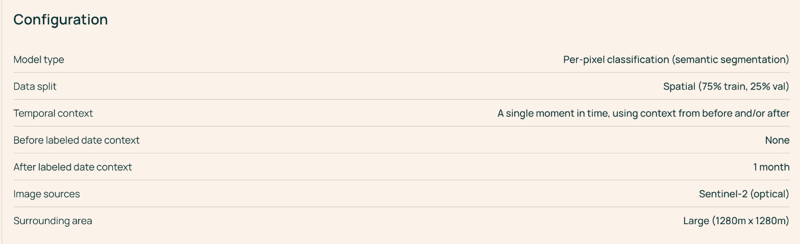
This example uses per-pixel classification at a single point in time, using imagery from up to one month after each labeled date, with Sentinel-2 imagery and a 1,280 m × 1,280 m surrounding area. For guidance on each setting, see Model Fine Tuning.
3. Evaluate model performance
When training finishes, Studio evaluates the model on the validation labels that were set aside from training. Classification models report overall accuracy, mean F1 score, per-class metrics, and a confusion matrix. Regression models report error metrics such as RMSE, MAE, and R².
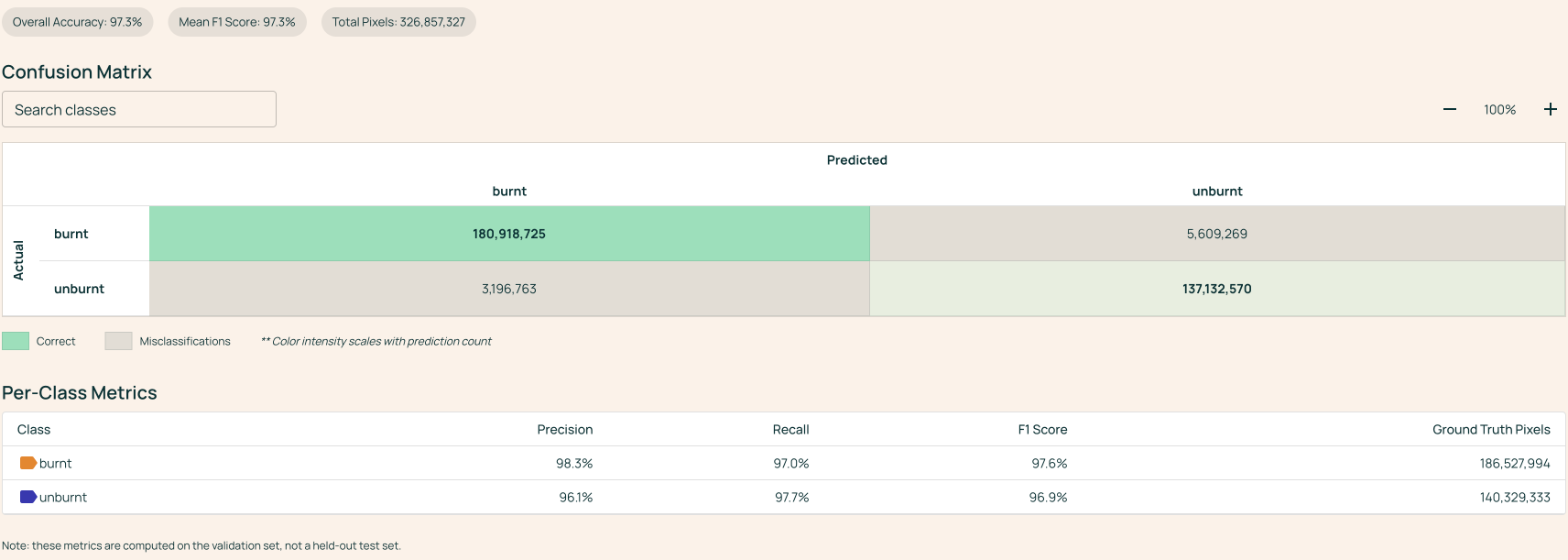
The confusion matrix compares the model's predictions (columns) with the labels (rows). Values on the diagonal are correct predictions, and values off the diagonal show which classes the model confuses. In this example, the model reached 97.3% overall accuracy, and its most common error was missing burned area: predicting unburned where the label was burned (about 5.6 million of 327 million pixels).
4. Fix errors and retrain
Click any cell in the confusion matrix to open those examples in the Data Viewer. The map shows exactly where the model made that mistake.
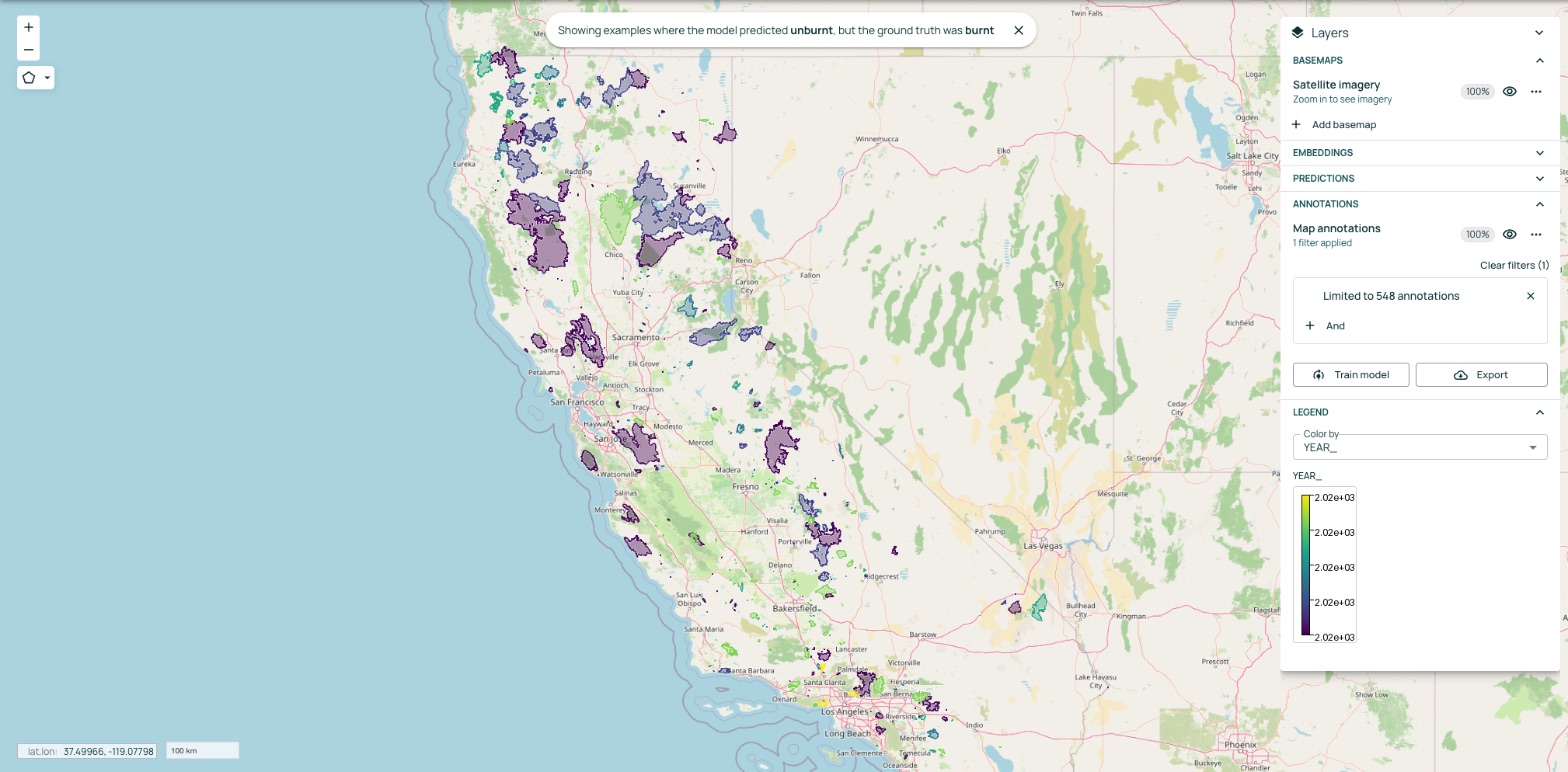
Use this view to decide where the model needs more information. Common fixes include adding labels in areas where the model struggles, correcting mislabeled data, and adding examples of classes the model confuses. Then select Train model to fine-tune a new version and compare its results with the previous one.
5. Run predictions
Run your fine-tuned model over any area of interest by drawing a polygon on the map or uploading a GeoJSON file, then choosing a date range. Studio acquires the imagery and runs the model for you.
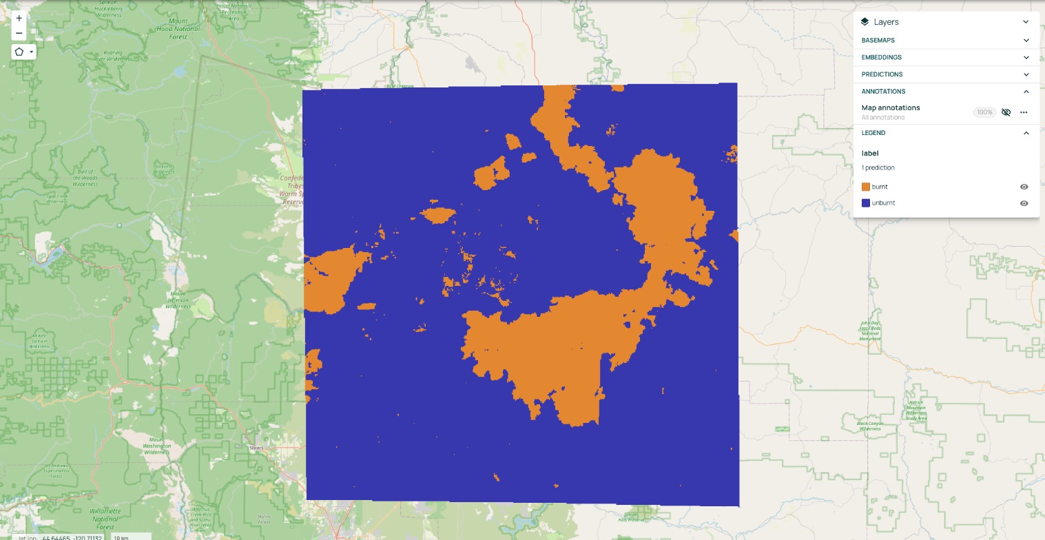
This example maps burned and unburned land across part of central Oregon for 2025.
6. Export your results
Download predictions as GeoTIFF rasters or, for vector outputs, GeoJSON files to visualize them and layer them with other datasets. You can also retrieve results programmatically through the Interactive OlmoEarth API Browser.